
By Hurley Gill • Senior Systems and Application Engineer | Kollmorgen
Servomotor-inertia ratios impact overall machine efficiency, and their use has evolved with servo-drive technology. So now, the newest digital servo-drive and feedback technologies can get higher inertia ratios while maintaining stable control to target velocities and positions. That can boost design efficiency, especially for dynamic applications such as indexing.
In bleeding-edge applications, it’s acceptable to design motor-driven machines for the best possible performance without considering operating cost. However, most industries need machines that perform well at the highest possible efficiency. Unfortunately, articles and other publications that reference servomotor and drive sizing often miss this important point.
Though mathematical solutions are well documented for mechanical systems, they don’t necessarily account for actual machine functions (or work to be done) and don’t account for specific control capabilities (or limitations) to help engineers pick the best motor, drive and feedback. But well-designed machines can slash power-utility payments—so justify deeper analysis of each machine axis. What’s more, when most of the used energy goes to driving the machine’s loads, total energy consumption goes down. That equates to a lower overall torque requirement—and often lets engineers pick motors for machine axes that are smaller and less costly as well.
Get better servo-system efficiency with appropriate inertia ratios
Efficient designs are increasingly valued for environmental and monetary reasons, so designers should aim to pick the best motor-drive-feedback system for the application, keeping in mind each technology’s advantages and disadvantages. This reduces the risk of failure (important for risk management) and makes the machine more practical, usable, competitive and sellable.
In this article, we explain one guideline to help engineers do this — a figure-of-merit, defined as a quantity based on one or more characteristics of a system or device that expresses design effectiveness. Here, the figure of merit we use is the inertia ratio. Basing design work on inertia ratios helps engineers minimize energy demand for dynamic high-speed machines—whether the axes are direct-drive or have mechanical power-transmission devices.
Servo-system inertia ratio basics
What is a servo’s inertia ratio or mismatch (abbreviated J_load:Jm)? Simply put, this inertia ratio helps express overall controllability and risk of servocontrol instabilities. It’s an important figure for all closed-loop (servo) applications, particularly dynamic ones. The two terms of the moment-of-inertia ratio or mismatch for a rotary servo system are:
1) The load’s total moment of inertia, J_load. Here, the inertial load is that from all the axis’ components (reflected through mechanisms when applicable) and summed at the motor’s shaft.
2) The motor’s moment of inertia, designated here as Jm.
Inertia mismatch is not a concrete number or even a concrete range for every application. That said, there are some ratio ranges that are generally applicable to specific applications and machine designs.
Consider how many technical manuals say that an ideal inertia mismatch is 1:1. Well, this is the ideal mismatch to maximize power transfer and minimize potential control issues … while the acceleration and deceleration energy is evenly split between
J_load and Jm (where J_load = Jm and
J_total = 2·J_load). However, the most efficient dynamic applications maximize acceleration of the load’s inertia (within the confines of axis stability, controllability, accuracy and repeatability). So for a fixed J_load, the most efficient version of a machine gets maximum acceleration with the lowest possible Jm … and not a minimal matched J_load.
History of this factor-of-merit
When servo drives were first developed, they were analog. Designers tuned servocontrol loops by hand, adjusting resistance and capacitance-decade boxes in a lab with an oscilloscope. It was hard to fine-tune servocontrol loops to customer-specific mechanisms, so drive manufacturers sold motor-drive combinations with a preset compensation (COMP) to get axis stability for most applications. The manufacturer’s COMP usually assumed the OEM’s machine needed an inertia mismatch J_load:Jm of 1:1, because this ratio has the least potential for axis instability.
Picture a gearhead-fitted servomotor driving an axis. The gearmotor exhibits backlash between the gear teeth. Here, a standard COMP must maintain current, velocity, position and loop stability no matter the reflected inertia—even though the motor sees the maximum load’s total-reflected inertia as well as its minimum whenever the drive teeth transition between driven. The closer the axis stays to the presumed inertia mismatch of 1:1, the more likely the control maintains axis stability during operation.
That’s why for years, drive manufacturers setup COMPs to work with standardized inertia mismatches, and then advised OEMs to build their machine axes to stay within those inertia-mismatch ranges. A 1:1 J_load:Jm mismatch (based on the maximum power-transfer equations) lets designers build axes with simple gain adjustments on current and velocity loops, and an external position loop when applicable. Such COMPs perform well on machines with J_load:Jm mismatches from 1:1 to 3:1 or even 5:1. Some applications could even use standard COMPs with machine mismatches up to 8:1 or even 10:1. But beyond that, machines needed special compensation—and in the past, manufacturers had to write custom COMPs to accommodate higher inertia mismatches.
Despite the limitations, a standard inertia mismatch with a useful inertia range lets designers use servo-systems to get machine stability … and keeps manufacturers and OEMs from going crazy because of instability issues.
Most analog drive manufacturers used a 1:1 inertia (maximum power transfer) ratio for standard COMPs—though their suggested J_load:Jm inertia mismatch range sometimes varied with their experience, market, and the drive’s control-loop transfer-function capability. Inertia ratios of 3:1 to 5:1 were common, and ratios of 1:1 to 3:1 were typical for many high-speed indexing applications. Fixing the factor-of-merit to an inertia mismatch of 1:1 was and still is a way for drive manufacturers to maximize customer satisfaction and sell complicated products with minimal risk of control instabilities. Even most stepper-motor manufacturers advertised such functionality—touting their drives as simple components using a specific inertia ratio. Everything worked fine for these open-loop stepper systems as long as the application’s load inertia and friction were close to (or less than) those in published capabilities.
The problem? Applications can’t perform efficiently when they’re pinned to one mismatch. In fact, mismatch in the most sophisticated systems changes with the axes’ mechatronics and dynamics—including friction, stiction, external loading, backlash, compliance and stiffness; loads, mechanism inertia, feedback resolution, the number of moving bodies between the load and motor, and design natural frequencies; the motor’s drive PWM/SVM and update rates; and the controller’s separate update rates, when applicable.
Few of these factors get consideration in inertia-mismatch J_load:Jm calculations, because accounting for them complicates controls—plus these factors weren’t typically considered in the past. But now that’s changing … and with increasingly sophisticated controls, OEMs now have options to build machines that operate with better performance and efficiency.
New capabilities for servomotor inertia-ratio flexibility
When digital drives for servomotors first came to the marketplace, they vastly improved compensation flexibility, filtering and the ability to program motion profiles. Even so, reliance on the old figure-of-merit (inertia mismatch) didn’t change. Plus, early digital servo drives weren’t always well suited to replace analog drives.
However, today’s digital servo drives have faster processors (FPGAs), faster update rates, and enhanced compensation methods and models. What’s more, in most applications, higher-resolution feedback devices in excess of 221 to 227 bits per revolution make for a more-responsive servo system. For example, axes that once got feedback resolutions of 212 to 216 counts per mechanical revolution can now get the same counts in a fraction of the previous time or displacement. That allows higher control-loop gains and higher bandwidths to catch and control possible instabilities before they have a chance to become unstable.
Today’s newest servo drives pair well with mechatronic designs and have control capabilities that are so good that engineers can assume the effects of J_load:Jm are minimal for even dynamic applications. That lets engineers set inertia ratio ranges to maximize energy efficiency and minimize instability concerns (within reason, and maintaining good risk management), even for high-speed indexing-type applications.
Potential energy savings for servomotor-driven designs
Sometimes end users quicken manufacturing processes to get higher throughput, or speed up machines for faster response. Here, machines must make those quicker moves and respond to all commands and disturbances while maintaining output-product quality.
Consider a factory floor where products are machined or otherwise processed. Sometimes, it’s impossible to quicken a specific process, so plant engineers try to hasten the material-handling stations—the axes that move parts to and from workstations—instead. This increases the axes’ peak horsepower draw during acceleration and deceleration (from the baseline production rate) by the product of the new increased speed and torque.
To illustrate, let’s explore how this works for high-speed indexing applications and what the inertia-ratio sweet spot becomes for the lowest power requirements, expressed as the percent energy saving versus inertia ratio.
Dynamic indexing application example
Consider several high-speed indexing applications, of both direct drive and mechanically advantaged (belted in this case), accomplishing completely different jobs in different industries and markets, with low friction and no external loading. Assume we fix process time to force the machine to make specific moves in less time (as often seen in the real world). Say for three situations, we set index times and have fixed peak torque T(peak) at about 1.6 x T_rms; about 2.0 x T_rms; and about 2.4 x T_rms.
Once we calculate maximum traverse rpm N and the RMS equivalent velocity N_rms for each motion-profile, they are constant for that specific motion-profile regardless of the inertia mismatch or ratio. The relative percentages of energy savings for all three situations are basically equal. That’s because the theoretical maximum power savings possible for each case falls within a few percent of each other. To simplify our next round of calculations, let’s only consider the second situation, with T(peak) = 2.0 x T_rms.
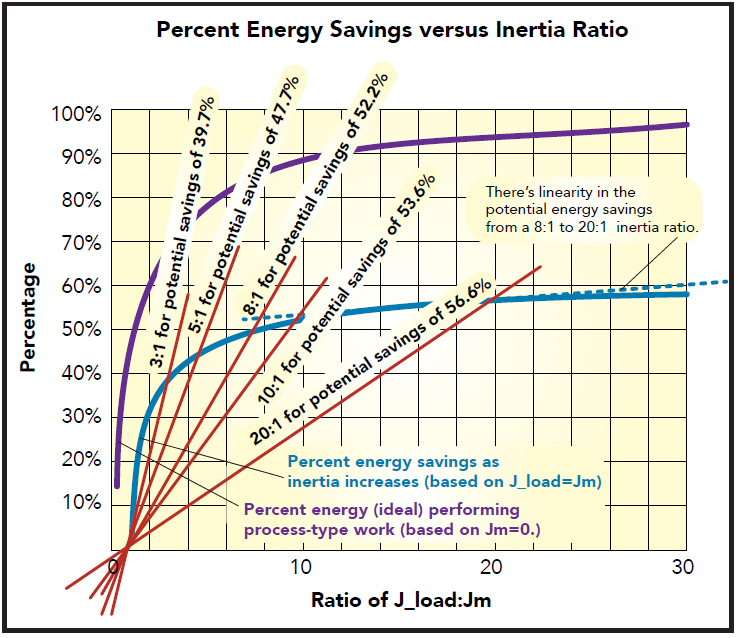
Note that a 3:1 inertia ratio J_load:Jm over the baseline 1:1 ratio can present an actual energy savings potential of approximately 39.7%, as seen in the plot, Percent EnEnergy Savings Versus Inertia Ratio. Also consider the chart titled, Energy Savings as a Function of Inertia Ratio, and note how a 5:1 ratio makes for actual energy savings exceeding 47.6%—about 80% of the theoretical maximum available savings. Likewise, an 8:1 ratio makes for actual energy savings exceeding 53.6% that equates to 87.5% of the theoretical maximum savings—a pretty significant energy savings over the baseline 1:1 inertia mismatch.
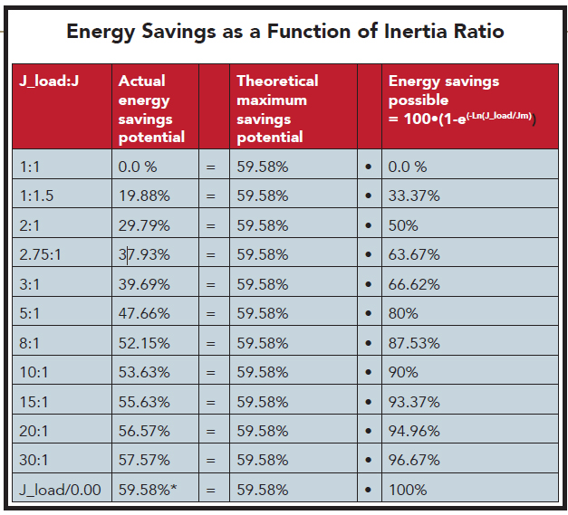
Reconsider efficiency’s relationship to the J_load:Jm ratio. Identifying an ideal inertia ratio or ratio range for maximum energy savings is highly subjective, but users generally want to save as much energy as possible. So say we aim to get 80% to 90% energy savings of the maximum available to upward of 95% (in the chart’s fourth column) of the ~60% (chart’s third column). This means the target J_load:Jm range is 5:1 to 20:1 for most of these dynamic applications.
90 to 95% is even better energy savings, which translates into an inertia ratio range of 10:1 to 20:1. But even an 8:1 ratio presents an energy savings potential of 87.5% of the theoretical maximum available. Many new motor-drive systems today can accomplish these dynamic applications with little additional risk of instability.
These energy savings also directly impact the motor sizing/selection and cost, as traverse velocity (N) and N_rms are fixed by the motion profile. Therefore, the required application torque (T_rms) is smaller, so the machine designer can use a smaller (and less costly) motor, if it’s available.
Energy savings for servomotor inertia ratios: Calculation caveats
Reconsider the figure titled, Percent Energy Savings Versus Inertia Ratio. Actual energy savings for any inertia ratio (relative to 1:1) as a percentage of the theoretical maximum savings equals the theoretical maximum savings potential (Jm = 0)*(1-e(-ln(J_load/Jm)), where theoretical maximum savings potential (Jm = 0) = 59.58%. So to get the percentage of actual energy savings potential with an 8:1 ratio (versus a 1:1) we use:
Actual energy savings potential (with an 8:1 ratio) = 59.58%*(1-e(-ln(8))= 59.58%*0.875 = 52.1% … same as that from actual motion-profile calculations.
In a similar way, if we have a 2:1 inertia on an axis and want to estimate actual energy savings, if we go to a 15:1 inertia ratio for a high-speed indexer, we can estimate it from the chart titled, Energy Savings as a Function of Inertia Ratio. Use the chart’s second column to get:
100 * (55.63%-29.79%)/(100-29.79)
= 100 * 25.84/70.21
= 36.8% energy savings.
The same chart reveals that going from a 1.5 to a 15:1 ratio would make for a 44.6% energy savings.
In contrast, the percent actual energy increase of going to a 3:1 inertia ratio versus the present ratio of 10:1 (for example, due to product obsolescence) is approximated from chart’s second column as follows:
100 * (53.63%-39.69%)/(100-53.63)
= 100 * 13.94/46.37
= 30% energy increase.
Here’s one last exercise to illustrate the point. Assume we have a mechanically advantaged mechanism (a gearmotor) with an initial goal of a 10:1 inertia ratio—Jratio. Then the gear ratio is:
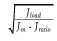
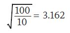
So if Jload (listed J_load elsewhere in this article for readability) equals 100 kg-cm2 and Jm is 1.0 kg-cm2, then the gear ratio is:
After that, the designer should select a motor with sufficient speed and torque capabilities (T_rms, N_rms, T_peak, and N_max/traverse) as well as the Jratio range. Then the designer should fine-tune the numbers and motor selection for final calculations and confirmation of the application’s design.
Cost savings summary
Proper motor-drive-feedback selection of a servo-controlled axis is perhaps the single most significant savings element a machine designer can make for reducing the user’s operational energy cost. Today’s digital servo drive technologies have significantly higher feedback resolution than available just a few years ago … and that’s made for stable and repeatable axis control due to higher overall bandwidth capability. This, plus good mechatronics design (in harmony with the work done by each machine axis), lets the designer dramatically increase the J_load:Jm factor-of-merit … particularly compared to what was available more than a decade ago.
In short, machine performance and axis controllability (ease of servocontrol-loop tuning) generally increase as the inertia ratio approaches 1:1, but higher inertia ratios let the designer lower manufacturing, operating and possibly even machine cost.
Because today’s products and servocontrol capabilities largely address concerns about control stability, designers can focus on optimizing inertia ratios for higher energy efficiencies. More specifically, designers can pinpoint the range for an inertia ratio range to get the most efficient power use … usually a range of 8:1 to 20:1, with even higher ratios for some applications.
Case in point: Most mechanically advantaged indexing applications can use today’s advanced servo drives paired with high-resolution feedback and low-inertia servomotors to get these energy savings. However, many high-speed indexers have a much smaller J_load whether mechanically advantaged or not. That’s not to say that a direct drive can’t have a much higher inertia ratio. In fact, it can … by orders of magnitude, usually limited only by the compliance of the steel components driving the load, machine-frame stiffness, feedback resolution, and available system bandwidth. However, the inertial load J_load of many high-speed indexer applications is much lower, often approaching today’s motor’s rotor inertia Jm for the comparable required torque.
Kollmorgen
www.kollmorgen.com


Leave a Reply
You must be logged in to post a comment.