By Hurley Gill • Senior applications and systems engineer | Kollmorgen

Please refer to part one and part two of this three-part series for background information on the functions and types of regenerative resistors for servo applications.

Let’s now consider the worst-case deceleration of an axis needing to reach a zero velocity for a p-stop or e-stop. This simple exercise will identify the necessary regen resistor based on an Er(sf) value without delving into the more complicated calculations for a multi-axis system or even single axis required to make multiple decelerations.

Design assumptions: A 3Ø 480-Vac source powers a rotary electric servomotor driving a horizontal axis needing to decelerate to zero RPM. So, normal application operation for the motor and drive yield:

     Trms = 20_Nm and Tpk = 50_Nm at Ipk = 28_Arms
J_load = 1_kg·m² and Pc_req = 1041W
Ppk_req = 1,150 W.

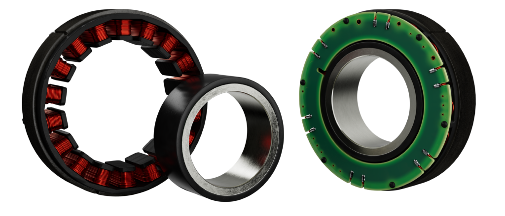
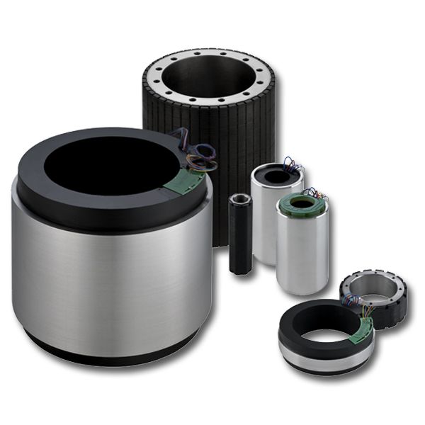
Selected motor and drive performance values: Let’s assume we selected a frameless brushless motor with a Kt(rated temp) = 2.19_Nm/Arms; Kb(25°C) = 133_Vrms/kRPM; Jm = 0.00304_kg·m²; Tpk(motor) = 76.1_Nm; Rm(L-L) = 1.41 Ω (for Rm cold or ambient temperature).

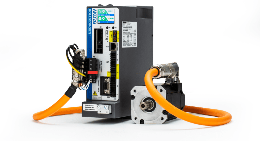
Assume we have selected a servo drive having an Ic = 12_Arms, Ipk(drive) = 30_Arms, DC-bus capacitance = 470µFd, Vmax(fault) = 840 VDC, an internal regen RBint = 100 W and 33 Ω. Regenerative output Regen(c)_output(480vac) = 6kW and Regen(pk)_output(480vac) = 21.4kW for 1sec; Regen(ext) = 33_ohm (Ω).

Now assume our stop-function (sf) linear deceleration is Tpk = 50_Nm at Ipk = 28_Arms for t_dec = 1.2_sec. For a stop-function analysis, we need to use the data from the application’s motor-drive selections to minimally identify five values:

Irms(application) = Trms/Kt(motor) = 20_Nm ÷ 2.19_Nm/Arms ≅ 9.13_Arms

Nmax (maximum velocity) = 570rpm, where the highest kinetic energy resides; typically, this will be the maximum velocity (just prior to any possible stop-function (sf)) with largest mass, with the least friction and any external loading aiding (-) or resisting (+) axis’ ability to stop.

Total inertia (J_total) of the axis — i.e. all reflected inertia & otherwise (J_load) at the motor plus motor’s rotor inertia (J_motor). J_total = J_load + J_motor = 1_kg·m² + 0.00304_kg·m² = 1.00304. Note with a J_load / Jm = 329:1 mismatch, this must be a directly driven load.

Friction torque (Tf) at the motor … noting that if Tf is relatively small, it’s often assumed that Tf = 0_Nm.

Any external torque (T_ext) at the motor during subject stop-function deceleration; for our example: T_ext = 20_Nm (positive (+) value meaning for this application: it adds to the E(k) making it harder to stop axis (as for a vertical axis trying to stop a downward move where gravity adds E(k) making stops more difficult).

The next step in our analysis is to identify the desired stop-function deceleration-time t_dec. Note that this t_dec value is typically that required to meet some customer stop-function requirement and/or that which is dictated by available drive-current limits — such as the drive’s I2t (I²t) foldback algorithm. Identifying the most suitable stop-function deceleration time will likely take multiple calculation iterations. For deceleration times demanding Ipk(drive) for more than the available time as a function of the drive’s I²t algorithm, the Ic(drive) is often used. Otherwise, Ipk(drive) or Ipk(motor) becomes the limit. For our example here, Ipk(drive) is available for the t_dec = 1.2_sec.

Note that for linear applications, it’s necessary to replace rotary-inertia J units in kg·m² with mass M units in kg … as well as velocity ω units in radians/sec with velocity V units in meters/sec.

Er(sf) = E(k) – E(el) ± E(ext-f) – E(f); that is: kinetic energy less losses ± any external forces, where each unknown is calculated & identified, by the axis’ stop-function (sf) conditions. For this example:

E(k) = Energy(kinetic) = ½(J_load + J_motor) ωm² = ½(1.00304_kgm²) (570rpm/9.55) ² = 1786.62_joules

E(el) = Energy(electrical losses) = 3(I²_dec x Rm/2) t_dec. = 3(28² x 1.41/2) x 1.2 = 1989.8_joules

E(ext-f) = Energy(external forces) = T_ext x Δωm/2) t_dec = (+20_Nm x 570rpm/2/9.55) x 1.2_sec = 716.3_joules

E(f) = Energy(friction) = (Tf x Δωm/2) t_dec … and because Tf is relatively small, we assume E(f) = 0_joules

Hence Er(sf) = ½(J_load + J_motor) ωm² – 3(I²_dec x Rm/2) t_dec ± (T_ext x Δωm/2) t_dec) – (Tf x Δωm/2) t_dec.

So Er(sf) = 1786.62_joules – 1989.8_joules +716.3_joules – 0_joules = 513.12_joules.

Because the calculated Er(sf) > 0, we need to determine whether the drive’s DC bus has the capability to absorb the 513.12 joules returned to the DC bus. The DC-bus capacitance E(caps) = Energy(additional capacity) = ½ C (VDC²_max(fault) – VDC²_bus). For our design, that’s equal to ½ × 470µFd × ((840-1)² – (480vac√2)²) = 57.13_joules.

We first need to verify whether the drive’s DC bus can absorb the returned joules through its internal regenerative resistor capabilities — with that for our selected component expressed as RBint = 100 W and 33 Ω for a t_dec = 1.2_sec … and E(int-reg) = 120_joules.

That means Er(sf) – E(caps) – E(int-reg) = 513.12_joules – 57.13_joules – 120_joules = 336_joules … so Er(sf) – E(caps) – E(int-reg) > 0. That in turn means that an external regenerative resistor is required with a minimal dissipation capability > 513.12_joules … or at the very least, we need to extend the time over which deceleration is allowed to occur.  One caveat here: For a stop function event, we cannot guarantee any DC-bus capacitance storage capability — which is why E(caps) is not subtracted from Er(sf) for the final determination of minimum requirements.

Calculated wattage for the stop function: Ppk_req(sf) = Er(sf)/t_dec = 513.12_joules/1.2_sec = 428 W.

Now let’s calculate the required minimum continuous power requirement. The minimal continuous power requirement is Er(total) / t_total; however, we need the maximum peak requirement for the selected motor and drive based on a specific event — the stop function — and not for the continuous power requirement defined by the Application results (i.e. Pc_req = 1041W) based on normal axis operation (motion profile).

The continuous power requirement defined by the application results gives Pc_req = 1,041 W based on normal axis operation executing the actions plotted on its motion profile. However, here we are looking for the maximum peak requirement for the selected motor and drive based on a specific event— the stop function — and not the continuous power requirement.

Note: Any Pc_req calculated from a stop-function motion profile will be bogus and of little value … unless the specific stop-function is modeled with Trms, Nrms, and Nmax (RPMs) based on worse-case normal operation appropriate for the application and motor-drive selection. The latter type of modeling isn’t typically done, because that information is determined during the original sizing. A slightly altered approach to modeling an axis’ stop function is to use an equivalent motion-profile segment for normal operation just prior to the defined stop function under evaluation — including RMS continuous conditions, maximum velocity, and any external loading. This will help determine if there are any I2t foldback algorithm issues.

For our example, peak regen power requirement with a Pc_req = 1,041 W, Ppk_req = 1,150 W, and Ppk_reg(sf) = 428 W. So for this application example, Pc_req is actually the dominant requirement for regen wattage selection. The standard regen resistor selection for the proposed drive is 33 Ω with wattage ratings of 250, 500, 1,500, and 3,000 W. A 33-Ω 1,500-W regen resistor (assuming Ppk_resistor = 10 x continuous) is our best selection from standard manufacturer offerings.

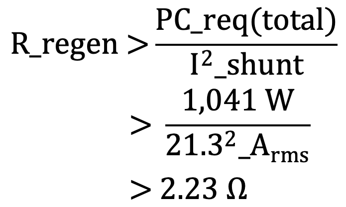
So does the 33-ohm 1500-W regen resistor meet all the application’s conditions? Well, let’s find out. The selected regen resistor’s maximum resistance that will continuously allow the DC bus to be maintained under its maximum value — VDC_max(fault) — is determined by:

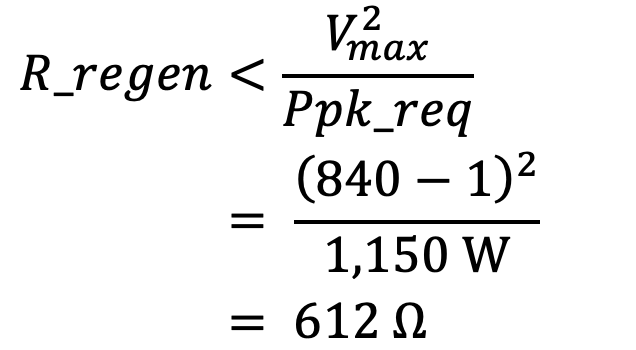
However, for the selected next size up standard resistor having a capability: 1,500W,  R_regen(Ω)  must be less than 469 Ω.

Assuming we choose the 1,500-W 33-Ω regen resistor, the maximum possible regenerative shunt current I_shunt(Rmax) limited by the resistor’s peak capability is:

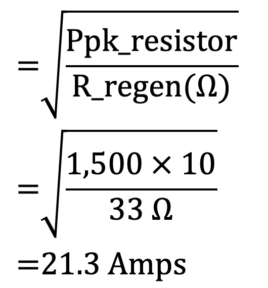
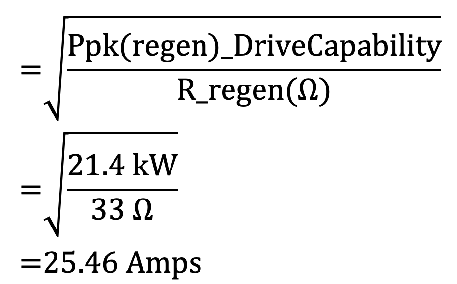
With this selected regenerative resistor, the maximum possible regen shunt current I_shunt(Drive-max) is limited by the drive’s capability — Given : Regen(pk)_output (480 Vac) = 21.4 kW for one second — and is:

The selected regen resistor’s minimal resistance shouldn’t exceed either the regen resistor’s shunt-current capability … or the drive’s maximum regen shunt-current capability. So I_shunt is equal to the lesser value between I_shunt(Rmax) and I_shunt(Drive-max).

However, for the chosen standard resistor having 1,500 W and 33 ohms, R_regen(Ω) should be larger than 3.3 Ω.

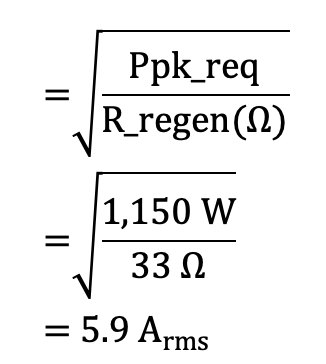
Pursuant to data from previously calculated requirements, the regen peak-current requirements I_pk(Reg-app) for the application and selected 1,500-W 33-Ω regen resistor is:

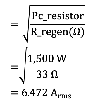
Given this selected resistor, the resistor’s continuous current capability Ic(Reg-Res) is:

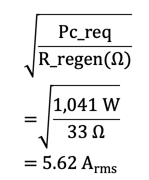
Pursuant to the given data (from previously calculated requirements), the regen continuous current requirements Ic(Reg-app) for the application and the selected 1,500-W 33-Ω regen resistor is:

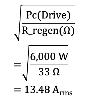
The drive’s continuous regen shunt current capability Ic(RegenCapacity of drive) —  based on a Regen(c)_output (480 Vac) of 6,000 W with the selected 1,500-W regen resistor is:

Finally, we run through the final confirmation of our regen-resistor selection.

• Pc_resistor (1,500 W) > Pc_req (1,041 W)
• Ppk_resistor (1,500w x 10) > Ppk_req (1,150 W)
• R_regen = 33 Ω — is a manufacturer’s standard offering for the selected drive.
• R_regen = 33 Ω < 610 Ω & < 469 Ω for the selected 1,500 W resistor
• R_regen = 33 Ω > 2.3 Ω & > 3.3 Ω — with the latter presenting the lesser peak shunt current.

So does the does the 33-W 1,500-W regen resistor meet all conditions?  Indeed, the selected regen resistor meets all conditions and is a reasonable choice.